Key Terms

 

o       Measure of asymmetry (skewness)

o       Skewness

o       Moment (about the mean)

 

Objectives

 

o       Recognize the definition of skewness

o       Use skewness to characterize the asymmetry of a data set

 

Lesson

 

In addition to measures of central tendency (which quantify the "middle" of a data set) and dispersion (which quantify the "spread" of a data set), measures of skewness are also helpful in characterizing data. A measure of asymmetry (or skewness) quantifies asymmetry in a data set (how much the data is "skewed" to one side of the mean). This lesson focuses exclusively on what we will call "skewness," but other higher-order measures can also be defined and used to characterize data (among these is kurtosis). For the purposes of an introduction to statistics, however, measures of central tendency, dispersion, and skewness go a long way in providing an extensive statistical description of a data set.

 

Skewness

 

Skewness is a measure of the asymmetry of a data distribution. Compare the data distributions below, which we also examined briefly in a previous lesson.

 

 

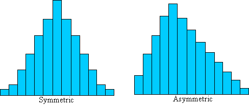
The distribution on the left is symmetrically distributed-it is not "skewed" to either side. The distribution on the right, on the other hand, is asymmetric--it is skewed to the left. We would like to derive a way to quantify the amount of asymmetry, which will allow us to further characterize a data set beyond just measures of central tendency and dispersion. Although we will not go through an extensive derivation of skewness, we can identify some of its characteristics and its relationship with the mean and variance. The skewness, γ, of a population containing N elements is defined as follows:

 

 

More generally, given a data set (x_i) with associated frequencies (f_i),

 

 

The term in the numerator is also known as the third moment about the mean μ. Note that the population variance, σ², for a data set with N elements is actually just the second moment about the mean μ.

 

 

In general, the kth moment about the mean is expressed as

 

 

Note that the skewness, γ, has a cubed term in the summation. The factor of 1/σ³ is always a positive number, so the skewness can be either positive or negative. As it turns out, given the above definition, data that is skewed to the right (that is, toward higher data values) has a negative skew, whereas data that is skewed to the left (that is, toward lower data values) has a positive skew. Thus, the skewness value not only gives us a relative magnitude of the asymmetry of the data set, but it also tells us in which direction the data is skewed. Consider the two depictions of skewed data sets shown below.

 

 

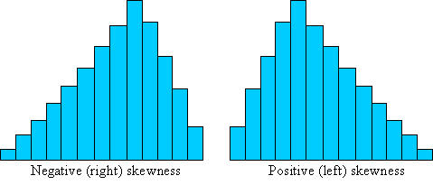
If a data set is symmetric, we would expect the skewness to be zero. Generally, we can then say that the frequency of some data value x_i is the same as the frequency of some other data value x_i + d_i, where x_i + d_i/2 (halfway between x_i and x_i + d_i) is the mean, μ. This algebraic representation simply states that every data value on one side of the mean has a corresponding data value equidistant from the mean (on the opposite side), and both of these values have the same frequency. Take a look at the symmetric distribution used above, which is depicted once again with an example pair of data values labeled.

 

 

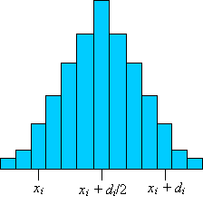
In addition to each such pair of values, there is the data value (and corresponding frequency) associated with the mean. For the mean value x_i = μ (even if it has a frequency of zero), the term in the summation is

 

 

Each pair of values as defined above corresponds to the two terms of the summation shown below.

 

 

Let's substitute our relationship μ = x_i + d_i/2.

 

 

Thus, the sum of the terms corresponding to pairs of values on either side of the mean is also zero. Extending this logic to the entire data set, the skewness of a symmetric set must be zero. This is the result we would expect.

 

Calculating the skewness for a given data set follows the same type of procedure as that required for calculating the variance. First, determine the mean and standard deviation of the distribution, then calculate the terms of the summation for skewness. The practice problems below provide you with the opportunity to calculate skewness for some example data sets.

 

 

Practice Problem: Calculate the skewness of the following (population) data set.

 

 

Solution: To calculate the skewness using the formula provided in the lesson, we must first calculate the mean of the data set.

 

 

Next, we can calculate the variance.

 

 

The standard deviation is

 

 

We can now calculate the skewness.

 

 

Note that if you use more accurate numbers (that is, numbers with more decimal places) than those used here, you may get a slightly different answer. In addition, the numbers you get for each step may differ even more significantly. A more exact answer (in some sense) for the skewness is 0.266. Regardless of the exact value, however, we can see that this positive skewness value indicates that the data is skewed to the lower values-we can also see this to some extent by inspecting the data table provided in the problem.

 

 

Practice Problem: Calculate the skewness of the (population) data set below.

 

{1.2, 5.4, 6.6, 7.1, 7.5, 7.7, 8.9, 9.5, 11.6, 15.2}

 

Solution: Our approach to this problem is generally the same as that of the previous problem, except that in this case we do not need to deal with frequencies. Let's start by calculating the mean, μ. Note that the data set has 10 elements.

 

 

Next, let's calculate the standard deviation.

 

 

Finally, we can calculate the skewness.

 

 

Again, you may find that your final result is slightly different if you use more accurate values than those used above (0.14 is a slightly more accurate result). The skewness of this data set once again indicates a case where the data "leans" toward the lower values (that is, values lower than the mean).