In this article, we expand our understanding to include multivariate data sets, thus allowing us in later studies how we can quantify relationships among data, for example. We focus primarily on bivariate (two-variable) data, but the concepts that we discuss can easily be extended to data with three or more variables.

 

Key Terms

 

o         Univariate data

o         Multivariate data

o         Bivariate data

o         Matrix

o         Scatterplot

o         Mean vector

o         Covariance

o         Covariance matrix

 

Objectives

 

o         Recognize multivariate data versus univariate data

o         Represent multivariate data using tables and scatterplots

o         Calculate descriptive statistics for multivariate data, including covariances

 

Let's Begin!

 

The types of data sets that we have considered thus far involve a single type of information, such as age, height, a particular measurement, and so on, for a population or sample thereof. This type of data is called univariate data, because it involves a single variable (or type of information). But data sets need not be limited to a single variable; more-complicated data sets can be constructed that involve multiple variables. We call this type of data multivariate data. Bivariate data, which is multivariate data with two variables. The principles that we discuss in terms of bivariate data can easily be extended to multivariate data with more than two variables. This article, then, considers some of the important concepts associated with multivariate (bivariate) data, with an eye toward later articles involving cross tabulation, regression, and correlation, for instance.

 

Representations of Multivariate Data

 

Univariate data sets can easily be represented as a simple list of numbers (although that list may get very long). This approach to multivariate data can quickly become cumbersome, however, especially when many different variables are involved. In such cases, a computer database may be the best way to record the data. For just two or three variables, however, a list can sometimes suffice. For instance, consider the following example data set containing information about age and income for a sample of a hypothetical city population:

 

{{24, $42,000}, {38, $29,000}, {52, $104,000}, {31, $37,000}, {42, $78,000}}

 

Tables are also a convenient way to represent data. The example data above can be represented in a table, as shown below. (Note that the data are arranged by increasing age; this is not a required approach, however.)

 

 

An equivalent representation that does not involve the trappings of a table is a matrix, which is similar to a table. A matrix has rows and columns like a table, but it is unlabeled. Matrices, like tables, can be used to display and organize data sets with many variables. A matrix representing the data set above is the following:

 

 

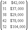
Note that each column of the matrix corresponds to a variable, and each row corresponds to a particular pair of data values (one for each variable).

 

When dealing with bivariate data, graphical methods can also be extremely useful. For instance, the scatterplot can serve as a means of displaying bivariate data and of more easily identifying trends and relationships in those data. A scatterplot for our example data above is shown below.

 

 

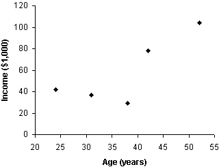
Making a scatterplot simply involves putting one variable on the horizontal axis and the other variable on the vertical axis of a standard two-dimensional graph. The points correspond to pairs of data values (one value for each variable). Thus, for instance, the leftmost point is at coordinates 24 (age-horizontal axis) and 42 (income-vertical axis). Multivariate data with three variables can also be expressed using a scatterplot, but a certain level with three-dimensional perspective drawing is required. Beyond three variables, scatterplots cannot be used.

 

 

Practice Problem: Convert the following data set into a table and a scatterplot. The variables correspond to two different measurements (the first variable is speed; the second is acceleration) for trials of a particular experiment.

 

{{46, 12}, {52, 14}, {53, 17}, {54, 18}, {59, 17}, {62, 22}, {64, 23}}

 

Solution: The data are organized according to increasing speed (the first variable in each pair), and we need not change this arrangement. Let's first create a table for the data. (No units are provided with these numbers, but typically, physical measurements have some associated units, such as meters per second for speed, for example.)

 

 

Next, let's create the scatterplot. You need not choose the exact ranges for the axes that are used below, but your choice should be such that the data points are all visible as well as (ideally) fairly distinguishable.

 

 

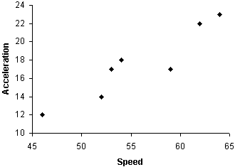
Note that we can easily identify a fairly clear relationship between speed and acceleration in these data: higher speeds tend to be associated with higher accelerations. We will learn in later articles how to quantify such relationships.

 

 

Descriptive Statistics for Multivariate Data

 

Calculating descriptive statistics for multivariate data is similar to doing so for univariate data. Here, we consider the mean and variance for multivariate data. The (arithmetic) mean for multivariate data is calculated in exactly the same way as for univariate data; the only difference is that several means must be calculated (one for each variable). This produces a mean vector, which is a set of n means corresponding to data with n variables. For instance, using our example age-income data from above, we calculate the means as follows. We'll assume for simplicity in this case that the data represent a population rather than a sample.

 

 

The mean vector μ is then

 

 

Thus, the mean age of the population is 37.4 years, and the mean income is $58,000.

 

Calculating the variance for multivariate data is slightly more complicated. Continuing to rely on our example data, we can easily see that age has a certain variance about its mean, as does income. Thus, we can use our variance formula from previous articles to express the variance of the age data and of the income data.

 

 

Notice that to avoid a huge income variance value, we simply calculated the variance of the incomes in units of $1,000--to calculate the actual variance, we must multiply this result (810.8) by the square of $1,000.

 

In addition to these variances, however, we might also be interested in how, for example, age varies with income or vice versa. The variance of one variable with respect to another is called the covariance, and it is defined mathematically as follows for two population variables X and Y.

 

 

Note that because of the definition, is the same as and the variance of a variable X is the same as the covariance . (The covariance of X and Y is sometimes written cov(X, Y).) Also note that the summation in the covariance can involve negative values. Finally, an estimator for the covariance of a sample simply involves replacing N with N – 1.

 

Let's calculate the covariance for the example age and income data.

 

 

We can write all the variance values in a covariance matrix, which performs a function similar to that of the mean vector (i.e., it groups the covariances in an orderly manner). The general covariance matrix for variables X and Y is shown below, followed by the specific covariance matrix for the example age and income data.

 

 

 

Practice Problem: Calculate the mean vector and covariance matrix for the following sample data.

 

 

Solution: The data are organized in columns; let's call the variable associated with the first column X and the second column Y. Let's now calculate the means for the data. Note that the data set is identified in the problem as a sample.

 

 

The mean vector is then

 

 

Let's now calculate the sample variances of the data.

 

 

The covariance matrix is then