How to Solve Linear Equations

Key Terms

o Linear function

o Slope

o Intercept

o Dependent variable

o Independent variable

o Linear equation

Objectives

o Identify the properties, graphs, and symbolic representation of a linear function

o Identify and solve linear equations

Linear Functions

A linear function is a type of function that involves a variable with an exponent of 1 (which is typically not shown, since x¹ = x, for instance). In simplest form, we can write a linear function f(x) as

f(x) = mx + b

where x is a variable and m and b are as-yet undefined constant values (i.e., numbers). First, let's look at a few plots of f(x) for various values of m. These plots are overlaid on the same graph below, which shows f(x) = x, f(x) = 2x, f(x) =3x, and f(x) = –x.

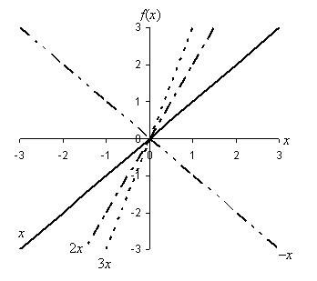
We can make some simple observations based on the plots of these functions in the above graph. First, note that the constant m apparently has the effect of increasing or decreasing the steepness of the graph. As m increases from 1 to 2 to 3, the line gets progressively steeper. Second, note that when m becomes negative (–1), the slant changes from upward (when going left to right) to downward. We call m the slope of the line and define it numerically as the difference in the vertical direction divided by the corresponding distance in the horizontal direction (this is sometimes called "rise over run"). The diagram below illustrates how we can calculate the slope of a line. Note that the particular horizontal distance that you choose is not important (it thus makes sense to choose a value that makes the calculation easy, however) because the slope of a line is the same everywhere.

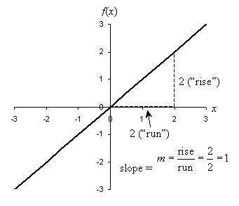
The slope of a line can range from 0 (horizontal) to positive or negative infinity (vertical). (Note, however, that a vertical line does not pass the vertical line test and is therefore not a function.)

Now we can attempt to understand what the term b corresponds to. Let's draw a graph that shows several linear functions with different b values: f(x) = x, f(x) = x + 1, f(x) = x + 2, and f(x) = x – 1.

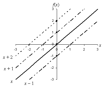
In each case, b corresponds to the value of f where the function crosses the vertical axis; this is the point (0, b) or, equivalently, (0, f(0)). We thus see that b is an intercept of the function. This intercept is usually called the y-intercept, because the horizontal axis is often called the x-axis and the vertical axis is often called the y-axis. Similarly, it is common to see a linear function written as y = mx + b; here, y takes the place of f(x). The variable y is often called the dependent variable because its value depends on the value of x. Likewise, because the value of x is allowed to vary freely, x (in this case) is often called the independent variable. At this point, then, we can now see what each part of a linear function is.

Practice Problem: What is the function g(t) corresponding to the following graph?

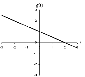
Solution: As the graph indicates, the function g(t) is linear. We can thus use the expression for a linear function in this case: g(t) = mt + b. Note from the graph that the line crosses the vertical axis at 1. We then know that b = 1. (If you are unsure about this, note that the line crosses the vertical axis at t = 0, and thus g(0) = 1. Use this to solve for b:

g(0) = 1 = m(0) + b = 0 + b = b

b = 1

This point is helpful to note.) We can then determine the slope by looking at the rise and run of the line. Note that the line decreases in height by 1 (and is thus negative) when t increases 2 units from the vertical axis out to t = 2. Thus, the slope m is

We can now write the equation of the line:

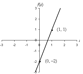
Practice Problem: Draw the graph of f(s) = 3s – 2.

Solution: We can draw a line on a graph if we know two points. Looking at the definition of the function, we know that the y-intercept (i.e., the intercept of the line with the vertical axis) is –2. Thus, we can draw a mark at the point (0, –2). We can find any other point using some arbitrary value of s; let's choose s = 1 for simplicity. In this case, f(1) = 3(1) – 2 = 3 – 2 = 1; we can therefore mark another point at (1, 1). Using a straight edge, we can then draw the line by connecting the points, as shown below.

Linear Equations

A linear equation is an equation that involves linear functions only. Each of the following is an example of a linear equation:

3x – 4 = 2

–8z = 2 – z

3 = d

We can find the solution of a linear equation (or "solve the equation") by applying the algebraic manipulations. Given an equation such as any of the examples above, our goal is to find an expression that identifies the value of the independent variable. Let's illustrate with the first example equation above; we want to solve for x. Simplify the expression by applying our rules of algebra and equality:

3x – 4 = 2 Given

3x – 4 + 4 = 2 + 4 Equality

3x + 4 – 4 = 6 Commutativity

3x + (4 – 4) = 6 Associativity

3x + 0 = 6 Inverse

3x = 6 Identity

Equality

Associativity

x = 2 Solution

The sequence of manipulations given above is exhaustive; as you gain facility with algebraic manipulations, you will not need to recognize each step above. You might more quickly process the equation as follows:

3x – 4 = 2

3x = 6

x = 2

Regardless of your approach, x = 2 is the solution to this equation-if we substitute x = 2 back into the equation, the equality will hold:

3(2) – 4 = 2

6 – 4 = 2

2 = 2

Other values of x, however, are not solutions and will lead to a contradiction. Consider x = 3:

3(3) - 4 = 2

9 – 4 = 2

5 = 2

Obviously, 5 ≠ 2, so x = 3 is not a solution to the equation. You might ask what a solution is graphically; let's look a little more closely at this. The equation 3x – 4 = 2 is actually an equation involving two linear functions, which we might call f and g. Thus, f(x) = 3x – 4 and g(x) = 2. Let's plot these functions on a single graph.

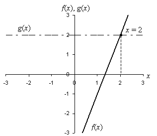
Notice that the solution to this equation is the x-value of the point at which the two functions cross. Thus, in addition to using a symbolic approach through algebraic manipulations, we can solve a linear equation by graphing as well (because this is a visual method, however, the accuracy of the solution can sometimes be suspect).

Practice Problem: Solve for q: 3q + 7 = –4 – q.

Solution: To solve for q, we must apply the rules of algebraic manipulations that we have learned so far. You may be able to easily perform these manipulations without the exhaustive justification given below, but these rules apply whether or not they are explicitly acknowledged.

3q + 7 = –4 – q Given

3q + 7 + q = –4 – q + q Equality

3q + q + 7 = –4 + q – q Commutativity

4q + 7 = –4 + 0 Inverse

4q + 7 = –4 Identity

4q + 7 – 7 = –4 – 7 Equality

4q + 0 = –11 Inverse

4q = -11 Identity

(4q) = (–11) Equality

q = Associativity

1q = Inverses

q = Identity

Again, you may be able to simply do the following:

3q + 7 = –4 – q

4q + 7 = –4

4q = –11

q =

By now, you should have a good grasp on the rules that allow you to perform these manipulations, and the following exercises will give you additional practice. Typically, however, as you begin to master algebra, you will rely more on the faster approach.

Practice Problem: Find the point of intersection of the functions f(x) = 3x and g(x) = –x + 2.

Solution: Two functions intersect at some x if the values of those functions at x are equal. Thus, we equate f(x) and g(x) and then solve for x, as shown below.

f(x) = g(x)

3x = –x + 2

3x + x = –x + 2 + x

4x = 2

(4x) =(2)