When you create a worksheet, you can decide what type of font you want to use. You can also decide the size of the font.

In the snapshot below, we've used Arial, size 12 font.  

You can clearly see how just changing the font type and size can alter the look of a worksheet. But let's learn how to do it.

The font tools can be found on the Home tab.

The currently selected font in the illustration above is Calibri, size 11. If no cell has been selected, this represents the default font. What that means is, if you were to click inside a cell and start typing, it would appear as Calibri, size 11.

To change the default font, make sure that no cells are selected, click the arrow to the right of box that says Calibri, scroll through your options, and click on one. You can change the font size in the same way.

To change the font in an individual cell or a series of cells, you must first select them. In the next example, we're going to select a range of cells. To do this, you can click in the top left cell, hold your left mouse button, and drag it down to the bottom right cell.

You can tell the cells are selected because of the dark line around them, the shaded blue area inside, or the highlighted row and column labels.

If you want to select cells that aren't in such close proximity to each other, you can press and hold the CTRL key while clicking on each cell, as in the example below.

Here cells A1, B4, and A6 have been selected.

You can change the font of selected cells the same way we change the default font.

Another way to change font of a selected cell is by clicking the tiny arrow in the lower right hand corner of the Font group. This will launch the Format Cells window, which looks like this:

From this dialogue box, you can also change the size. Just select a size from the Size section of the box.  

Now let's take another look at the Font group on the Home tab and discuss some of the other options associated with the appearance of our font.

To the right of the font size are two buttons. One is a large A with an arrow pointing upward, and the other is a smaller A with an arrow pointing downward. These buttons are just another way to change the font size. If you click the larger A, the font gets bigger. Click the smaller A, and the font gets smaller.

Below the font type are three buttons.

 Represents boldface. This is an example of boldface.

 Represents italics. This is an example of italics.

 Represents underlining. If you click the arrow to the right of the underlining button, you have a choice of a single underline (example), or a double underline (example.)

You can add borders to your cells by going to the Font group on the Home tab or by launching the Format Cells window. We'll cover both, of course, starting with the Font group.

This   is the icon for borders, located on the font group. To add a border around a cell, first select the cell. Now click the arrow associated with the borders button. A dropdown menu will unfurl.

Here you have a myriad of options. You can choose to create a bottom border, a top border, left border or right border, and more. You can even choose to remove all borders by clicking the No Border button.

In the following example, we've chosen to make a bottom double border.

To change the color of a border, click the Line Color option. This will show you a color palette from which you can choose.

Clicking More Colors allows you to create your own colors.

Now let's take a look at border options in the Format Cells window. You can launch this in a number of ways. The first we mentioned earlier--just click the arrow in the lower right hand corner of the font group, then click the Border tab. Another way to do it, is to click the arrow next to the Border button, then click More Borders. If you do it this way, the Format Cells window will open automatically on the Border tab.

Another way to launch this window is to right click on a cell, then select Format Cells. You may or may not have to click the Borders tab.

As you can see, the basic functions are identical to your options in the Border button dropdown menu. You can choose which side of the cell you want the border to be on, as well as a border style.

You can also select a color from this window.

Select the column(s) that you want to format. Go to the Home tab, and click the Format button in the Cells group. This will unveil a dropdown menu that looks like this:

Choose Column Width. A small floating window will open.

Want to learn more? Take an online course in Excel 2010.

The default column width is 8.43 characters. Here you can enter any value you wish and the entire column size will change accordingly. Keep in mind, though, that it reflects the number of characters that can be displayed.

But maybe you just want to make sure that the columns are wide enough to display all the content, but you don't want to take the time to count characters. Perhaps you aren't even sure how many characters there will be, but want to make sure the column will be wide enough anyway.

To do that, click the Format button and select AutoFit Column Width. Choosing this option will allow the column to expand to fit everything you type into it.

To change a default column width for every column in a worksheet, click the worksheet tab to make the worksheet active. To change it for the entire workbook, click a worksheet tab, then right click, and select Select All Sheets

To change the width of multiple columns, select the columns that you want to change, then drag the right side of one column to its desired width.

To change a row height, select the row(s) that you want to change, navigate to the Home tab, and click the Format button in the Cells group. Click Row Height.

A floating window will open that looks nearly identical to the Column Width window.

Enter a value into the Row Height box and click OK.

Note: It's important to remember that the cells you merge must be adjacent.

Below is an example of the cells we want to Merge. The cells have already been selected. As you can see, every cell in our example contains data.

To merge cells, select the cells to be merged. On the Home tab, click the Merge & Center Button . You can also click the arrow associated with the Merge & Center button for more options. Let's look at them.

The Merge & Center option will merge all the cells into a single large cell, with the data centered.

The Merge Across Option will merge each row of selected cells into a larger cell. For instance, in the example above, we'd have three cells as in the following example.

The Merge Cells option will merge all of the cells, but without centering the data.

The Unmerge Cells option will remove the merging in any selected cell that has already been merged. Please note, though, that any data that was lost in the original merge will not be replaced. It simply breaks the cell back up to match the current column widths and row heights.

Whenever you choose to merge cells, Excel 2010 will warn you about data loss with a warning window like this:

For example, we can have a number formatted like this in the worksheet:

 

But in the formula bar, it's still displayed like this: 

 

You can apply a number format to a cell by selecting the cell(s) that you want to format, then navigating to the Number group on the Home tab of the ribbon.

You will notice in the illustration above that the Number format type is General. That means it doesn't have any particular format. It's just a whole number without decimals and dollar signs. Click the area associated with this dialogue box to view your other options.

You have even more control over your options if you click the More Number Formats button at the bottom of the dropdown. This will launch the Format Cells window which we became familiar with earlier in this article. If the Number options are not already visible in this window, simply click its tab at the top.

In the dialogue box above, you can choose the type of number formatting that you want from the Category box. An explanation of how the formatting is used appears at the bottom of the dialogue box when you click on a specific type of number formatting.

 (You can also launch the Format Cells window by clicking the arrow in the lower right hand corner of the Numbers group.)

Creating Custom Number Formats If you go to the dialogue box above, and click Custom in the Category box, you can then create a custom number formatting based on an existing number format in MS Excel 2010. 

 

In the Type list, select the format that you want to edit and edit it in the Type box. Click OK to apply the format to a cell.

Align Cell Contents

You can align the contents of a cell by navigating to the Alignment group in the Home tab of the ribbon. Contents can be aligned to the top of the cell, the bottom of a cell, or the center of the cell. They can also be aligned left, right, and center, just like the text in a word processing program like MS Word. Below is an illustration of the Alignment group.

In the above example, the highlighted buttons tell us that the contents of our cell are aligned on the bottom edge, in the center between the left and right borders. The example below shows us how it looks in practice.

Cell Styles Your worksheets can contain a lot of data that might be hard to browse through. It helps to apply colors, different fonts and font sizes, etc. However, if you're new to MS Excel 2010, adding all these things may be difficult and time consuming.

So MS Excel 2010 comes with a number of predefined cell styles that you can apply simply by clicking a button. These are called Quick Styles. (Note: In Excel 2003, this feature was called AutoFormat.) They include options for changing: 

• Borders
• Number Formatting
• Background color
• Alignment
• Cell and row size
• Fonts

To see some of the predefined cell styles, go the Home tab and click the Cell Styles button . This can be found in the Styles group of the ribbon.

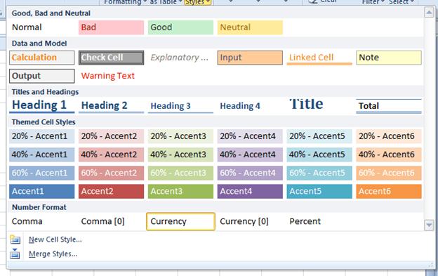
Clicking the Cell Styles button will unfurl a dropdown menu that contains a preview of a number of ready to use styles.

To use a Cell Style, select the cell (or cells) you'd like to apply it to, then return to this menu and click on an option.

You can restrict which formatting options to apply to a cell by right clicking an option and clicking Modify. You'll see a window which looks like this:

If you want to only apply a border and background color, you'd uncheck every box except Border and Fill. Click OK when finished.

Creating Your Own Cell Styles If you frequently use the same formatting options for the cells in your worksheets, you may want to create a formatting style to save you time. A formatting style is a collection of formatting choices. It may include, but not be limited to, font, font size, and color.

To create a new style, first format a cell with the selection of styles that you want. This is the easiest way to do it. Then click the Cell Styles button and select New Style.

We've chosen, for an example, to create a style using the format in this cell:

 

When we select new style, the Style window will open.

Clicking the Format button will launch the Format Cell dialog window where we can set options for our style like color, border style, font type and size, and more. Click OK when finished to close that window, then click OK in the Style window to save your new style.

Conditional Formatting Conditional formatting is a neat little feature of MS Excel 2010 because it helps you do your job better. Let's say that you're entering in employees' work hours into a spreadsheet. Your boss has told you to let him know if anyone exceeds more than eight hours in any given day. Did you know that you Excel can notify you each time this happens? You can program MS Excel 2010 to give you a "red flag" every time a certain situation exists.  

To apply conditional formatting, go to the Home tab and click the Conditional Formatting button as shown below:

. This will reveal a dropdown menu full of options.

 

Now, select the condition that you want MS Excel to notify you about. For this example, we're going to choose to be notified about a value of less than 15. So we'll click the Less Than option. This will launch a window in which we can enter our value. We're then going to use the dropdown menu on the right of this window to have our cells filled with red and a dark red text. Click OK when finished.

As you can see in the next example, a cell with the number 12 has been highlighted.

You can create your own conditional formatting rules by clicking the Conditional Formatting button and choosing New Rule. This will launch the New Rule window.

Select your desired options, then click OK.

Freeze and Unfreeze Rows and Columns

Freezing a row or column keeps it visible while you scroll. For instance, you may have column titles that you otherwise wouldn't be able to see if you scrolled down to the bottom a long document.

To freeze columns or rows, go to the View tab and click the Freeze Panes  button. This will reveal a dropdown menu.

Choose whichever option suits you best. You can choose to Freeze Panes based on the current location, to freeze just the top row, or to freeze just the first column.