XML

Click the Protect Workbook button, as shown in the example above. You should also note the information offered under "Permissions." This tells you the current security level of your workbook. In this case, anyone can open, copy, and change any part of it.

Clicking the Protect Workbook button reveals several options in a dropdown menu.

Mark as Final. This lets users know that this is the final version of the workbook and that it should not be edited. It can be edited still, of course, with the simple click of a button. The next example illustrates the message a user will receive upon opening an Excel workbook that has been marked as final. As you can see, the user can still edit the document by clicking the Edit Anyway button. He or she is simply "discouraged" from doing so.

To encrypt , simply type a password and click OK. Another window almost identical to this one will open, asking you to re-enter your password in case you made any errors. Click OK.

When a user tries to open an encrypted file, he or she will be asked to enter a password, as in the following example.

Entering the wrong password will result in a warning message like the one below.

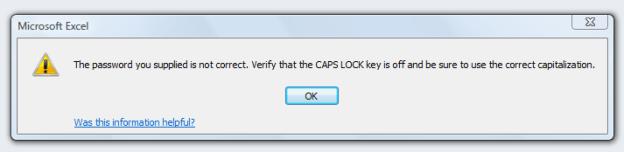
Just remember to write down any passwords you've created because once a file is encrypted, it cannot be recovered without a password.

Restrict Permission by People. You can use this option to choose which people can edit the workbook. It works by allowing users to sign in with their Windows Live ID, so each user you want to be able to edit the document must have one. If this is the first time you've used this option, you'll see a Service Sign-Up window which will walk you through the rest of the process.

When the service is set up, you can then select your permission options. In the following example, we've elected to restrict permission to the workbook. To the right of the one person who has permission, we can control the access level. There are three options, Read, Change, and Full Control.

You can set a date a permission expires on, so that after a certain date, the user can no longer access the workbook. You can also restrict whether a user can print the content of a workbook.

At the bottom of the window, you have the option of emailing the creator of the document to inquire about gaining greater access.

After you've added users, you can then click the Restrict Permission by People button and select an option from the menu. Options include Unrestricted Access, Restricted Access, and Manage Credentials.

Add a Digital Signature. Use this option to sign a workbook with a digital signature. This lets other people know that the workbook is genuine. Digital signature services can be purchased from third-party vendors, or you can create your own. Just be aware, however, that if you create your own digital signature it isn't as trustworthy as one provided by a third-party vendor and some recipients might not accept it.

Importing and Exporting Data

Microsoft Excel 2010 allows you to easily import and export data in a wide variety of different file types.

Importing Data

To import data, go to the Data tab. The import function are on the left side of the ribbon. Below is an illustration of the different buttons.

You can elect to import data from Microsoft Access, from the web, from a text file, or from other sources. To get an idea how the import process works, we'll walk you through the process of importing a text file.

To begin the process, click the From Text button as seen in the example above. This will start the Text Import wizard.

The first step is to select a suitable text file. (Note-this process imports plain text files rather than Word files.)

In the next step, you'll see a preview of the selected text file, and choose whether you want fixed width columns or if you want things like commas and tabs to tell Excel how to separate the text into new fields.

In the next step in the wizard allows us to show Excel where to cut the text into new fields. To do this, you'd drag the lines with the arrows on top to different places in the text. The lines will represent columns when the text is transferred to Excel. When you're satisfied with your selection, click Next to move on to the next step.

The next step allows you to select a data format for each column. The select columns are indicated by the black shading. You can choose a general format, a text format, or a date format. You can even elect to skip this step.

Click Finish when done.

The following is the way the text will look in our workbook.

Pivot Tables

A pivot table sounds more difficult and confusing than it really is. Most people say they don't like pivot tables, or they don't understand them. In truth, however, they're not that difficult at all.

Before you can create a pivot table, you must create a regular table. A pivot table is a data summarization tool used in Excel. You can use a pivot table to summarize data that you've added to a table. A table may be too large to allow you to analyze certain parts. A pivot table allows you to basically extract those parts (while leaving them in the table) to come up with figures, view the data, etc. Remember, tables were called lists in previous versions of Excel.

The best way to learn about a pivot table is to see how to create one.

We've created the table shown below. In tables, columns are fields and rows are records.

Select the table, then go to the Insert tab and click Pivot table, since we're working with a table. You can also create a pivot chart if you want.

The Table/Range is selected for you. Select New Worksheet, then click OK.

On the right, you'll see the Field list open up. This is a list of all fields in your table.

There are three kinds of fields:

Category fields are fields that you can group. In ours, we grouped category fields by department and position.

Data fields are fields that contain data that you can add, subtract, multiply, or divide. In ours, that's the salaries.

Arbitrary fields are fields that are neither data or category. The name field in our table would be arbitrary.

This is what you should now see on your screen:

If you look at your Pivot Table Field list on the right, and look to the bottom part, you see areas where you can drag and drop the fields. For example, we want Department to be a column header, so we're going to drag and drop Department down to the Column Labels.

We want Position to be a Row Header, so we drag and drop to Row Labels. We want the values shown in the table to be salary, so we will drag and drop that to Values.

Look at what that's created.

Now we can see the salary by department and by job description. If we had more than one salary per job description, it would total the salaries for us. Let's amend the chart to show you what we mean by adding another Account Manager.

As you can see, we added another Account Manager to our table.

The totals in the pivot table reflect both salaries.

Tip: Make sure there aren't blank rows or columns before you begin. Otherwise, Excel will only create the pivot table/chart up to the blank row or column.

With Excel 2010, there are some new Show As and other features to help you further sort and calculate data in a pivot table once you get it created. There are six calculations added to the Show Values As in Excel 2010.

Right now, we have a pivot table created from data from our regular table (formerly a list).

The values shown in the table are from the salary field. In Excel 2010, you can right click to see the Show Values As options.

To do this, select one of those values, then right click.

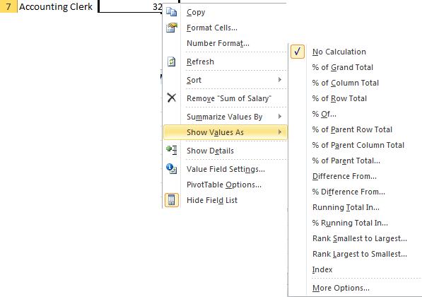
Now you can select how you want to show those values. We're going to choose to show them as % of Grand Total.

We can also right click and select Summarize Values By to tell Excel how to summarize the values in our pivot table.