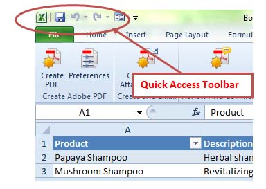
To add the Form button, click the arrow to the right of the Quick Launch toolbar and select More Commands. This will launch the Excel Options window, which can also be accessed by clicking Options on the File tab.
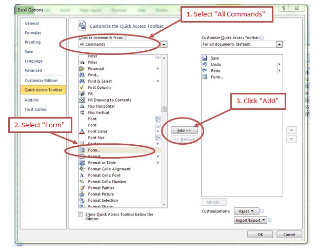
In the "Choose commands from" box, select All Commands, then scroll down through the list until you find Forms. Select it and click Add. When you are finished, click OK.

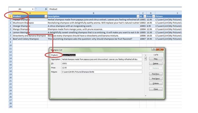
Entering data is as easy as selecting the correct field and typing. Use the Tab key to jump to the next field. When you are finished, press Enter. This automatically takes you to the next record. If you are at the end of the record list, it will create a new file.
Use the scroll bar or the Find Prev, Find Next buttons to browse through records.
Developing a Workbook
In this section, we're going to show you how to develop it further to fit your needs.
Format Worksheet Tabs


This will prevent you from accidentaly changing something, or an unauthorized person from editing it.
Choose a password, then select the items you'd like to protect. Click OK when finished.
Reposition Sheets
You can easily reposition worksheets by left clicking its tab in the lower left hand portion of the workbook and dragging it to the desired position. As you drag, a black arrow becomes active between the worksheet tabs, telling you where the worksheet will be place. Release the mouse to place the worksheet.
You can also right click on a tab and click Move or Copy.

You can choose to move the sheet between books, or within the same book, and position it before other sheets. You can also create a copy of the selected sheet. Click OK when finished.
Inserting, Deleting, and Renaming Worksheets

To delete a worksheet, right click on it and select Delete.
To rename a worksheet, right click on it and select Rename. The name of the worksheet will be highlighted in black. Type your new name and hit enter.
Copy Worksheets
Check the Create a copy box. You can copy sheets to different workbooks easily in this way.
Printing a Workbook
Printing a workbook is not quite as easy as printing a document in Microsoft Word. Setting it up to print in a way that is visually appealing and in the order you'd like takes some setting up. The rest of this section is devoted to helping you do just that.
The tools that will help you print your document correctly can be found on the Page Layout tab, while the Print button is located in File tab (Backstage View.)
Right now, let's focus on the technical aspects like choosing a printer and locating the print button.


If you don't have a printer installed, you can choose to add one.

Set Print Titles
 button opens the Page Setup window.
Here you can select a print area, as well as which rows or columns to repeat. You can also elect to print Gridlines, row and column headings, or in black and white and draft quality.
Use the Page order section to select the way in which Excel will print.
Headers/Footers
You can insert a header and a footer for each worksheet in your workbook. The Header/Footer  button is located on the Insert tab.
A header is any text or information that is entered into the top margin of a page, while a footer is the text and information entered into the bottom margin of a page.
When you click the Header & Footer button, the headers and footers become active in your worksheet.
Your worksheet will look like this. Below that is a zoom of the left and right sides of the Header and Footer Tools ribbon.


As you can see, a header is available for every page that will be printed. To enter a header, click it and start typing. In the example above, the header on the left is active.

You can use the tools in the Header & Footer Elements groups to add elements to your header or footer, such as a page number, the current date and time, a sheet name and even a picture.
Page Margins
The Page Margins  button can be found on the Page Layout tab. This allows you to set white space around the edges of your worksheets when you print them. (They don't normally affect how you work within a worksheet, at least not in the same way that page margins affect your documents in a word processing program like MS Word.)


Clicking the Print Preview button will show you an exact replica of what your worksheet will look like when printed. Click OK when you are satisfied.
Page Orientation
Page orientation refers to the long side of a page. For instance, if an ordinary 8 � x 11 sheet of paper is positioned vertically (that is with the shortest edge at the top and bottom), it's orientation is said to be in Portrait View. If the piece of paper is positioned so that the longest edge is on the top and bottom, it is said to be in Landscape View.


The Orientation  button can also be found on the Page Layout tab.
Page Breaks
The Page Break button is located on the Page Layout tab. When you enter a page break in this way, the place in your worksheet where the page break appears will be a dark dotted line, as in the following example.

Print a Range of Pages

Choose Print Selection, then enter the page range you'd like to print. In this case, we're going to print pages 2 through 7.
.Sharing Worksheets and Workbooks
There are several ways to share data and information located in your MS Excel 2010 workbooks with other colleagues, associates, or friends. The way you share depends on how you want to transmit the information, if the person you are sending it to has MS Excel, or if you just want to send a fixed version of a finished workbook by email. In this article, we're going to cover the ways that you can share your MS Excel 2010 workbooks.
Using Online Collaboration
An exciting new feature for Excel 2010 is the tight integration with the Excel 2010 web app. The web app is available from Microsoft Office Live, and requires a Windows Live ID to access.
The Excel Web App allows you to create and edit Excel files inside your web browser. This means you can access them anywhere, as long as you have an internet connection. You don't even have to have Excel 2010 installed on your computer.
Excel 2010 is, however, tightly integrated with the web app. You can easily access and edit documents in Excel and save them directly to the web.
What's more, the documents you create or even upload to the Excel web app are stored on SkyDrive, which is a "cloud service" provided by Microsoft. With Skydrive you can allow others access to these files for easy collaboration. You can even track changes someone else makes to your files in real time.

Protecting a Workbook
Even though you may be collaborating with other individuals, you may want to protect certain formatting options and pieces of information so that they cannot be inadvertently altered.


Change Versions of a Workbook
Excel allows you to recover previous versions of a workbook in case of emergency. To do so, go to Info on the File tab and then select Manage Versions.


Select a workbook and click Open.

If you'd like to keep the file, click Save As.
Set Up a Shared Version of a Workbook
You can use MS Excel 2010 to create a workbook that several users can work in simultaneously. All these users would create the workbook together, meaning this is very different than allowing users to edit a workbook.
To create a workbook that can be shared, go to the Review tab click the Share Workbook button.

This dialogue box shows you all users who have the workbook open at that time. If you want other users to be able to make changes at the same time, check the box at the top, under the editing tab. You should check this box for workbook sharing, then click OK.
Save the workbook. Go to the File Tab and save the file on a network location where other users can access and collaborate on it.
Note: If, after the workbook is finished, you'll want to merge all the copies together, click the Review tab and make sure track changes is enabled.
Merging Versions of the Same Workbook
Of course, when you have several users creating the same workbook, you're going to want to see the different versions that are created. Each user should save the workbook as a unique file name, then send the versions to you. You can then compare and merge the different versions with your own (the master version.)
Open the workbook that you want to use to compare against other versions.
The Merge Workbooks button is not available in the ribbon by default, but you can add it easily with the new customizable ribbon tools.


And there it is, on the extreme right of the above example.
Note: You can only merge a shared workbook with copies that were made from the same shared notebook. Also, all users must save a copy of the shared workbook with a file name that is different from the original workbook. However, all copies of the shared workbook should be located in the same folder.
Click the Compare and Merge Workbooks button and select the Workbooks you want to Merge. Click OK when finished.
Adding, Editing, and Deleting Comments
 . When a comment is made, a red wedge appears in the corner of the cell it's attached to.


Alternatively, you can navigate to the Review tab and click the Show/Hide Comment  button or the Show All Comments
  button. Use the Previous
  and Next
  buttons to navigate through the comments in a document.
If you select a cell that already has a comment in it, the New Comment button will change to the Edit Comment  button . Click this to be able to edit a comment.

The other way is to select the cell with a comment, going to the Review tab and clicking the Delete Comment  button.
Creating and Sharing Workbook Templates
A template is a worksheet or workbook that already had your preferred formatting such as font, font size, colors, etc. You can create your own templates in MS Excel 2010 easily and rather quickly. This part of the article will teach you how.
Creating a Template
Whenever you start a new workbook in MS Excel 2010, it uses the default template, which is simply a blank workbook with no formatting. The name of this default template is Book.xlt.
If you use various formatted worksheets regularly, you can create worksheet templates to make the process easier. The default worksheet template that MS Excel 2010 provides is named Sheet.xlt.
To create a template:
- Create a worksheet or workbook with the formatting that you want to be in the template.
- To save a formatted workbook as a template, go to the File tab and click Save As. The Save As window will open, asking you where you want to save the file and what you want to name it. Click on the Save As Type box and select Excel Template or Macro Enabled Excel Template. Click save and it will be stored as a template.

- To save a formatted worksheet as a template, create a template with just one worksheet. Format the worksheet as you want it for the template, then go tothe File tab, and select Template in the Save As Type box.
- Select the folder that you want the template to be stored in.